Deriving derivative and integral

To reach to here, we first had to work out the point slope formula and then figure out limits. Derivatives are very powerful. This post was inspired by doing gradient descent on artificial neural networks, but I won’t cover that here. Instead we will focus on the very own definition of a derivative.

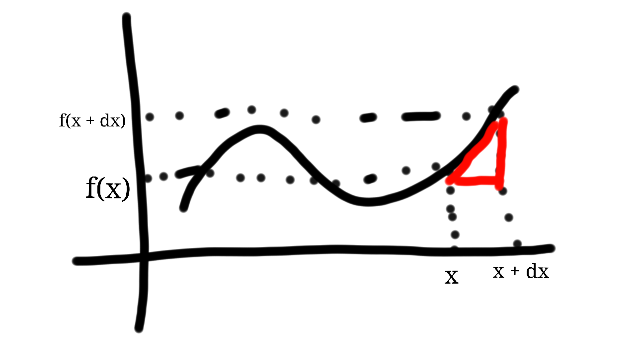
So let’s get started. A secant is a line that goes through 2 points. In the graph below, the points are $A = (x, f(x))$ and $A' = (x + dx, f(x + dx))$ .

To derive a formula for this, we can use the point-slope form of a equation of a line: $y - y_0 = \frac {y_1 - y_0} {x_1 - x_0} (x - x_0)$ .

Plugging in the values, we get: $f(x) - f(x + dx) = - \frac {f(x + dx) - f(x)} {dx} (dx)$ .

What is interesting about this formula using the secant is that, as we will see, it provides us with a neat approximation at f(x).
Let’s define $f_{new}(x, dx) = \frac {f(x + dx) - f(x)} {dx}$ . So now we have: $f(x + dx) = f(x) + f_{new}(x, dx) (dx)$ .

The limit as dx approaches 0 for $f_{new}$ will give us the actual slope (according to the definition of an equation of a line) at x.

So, let’s define $\lim_{dx \to 0} f_{new}(x, dx) = f'(x)$ . This slope is actually our definition of a derivative. This definition lies at the heart of calculus.

The image below (taken from Wikipedia) demonstrates this for h = dx.

Back to the secant approximation, we now have: $f(x + dx) \approx f(x) + f'(x) (dx)$ . This is an approximation rather than an equivalence because we already calculated the limit for one term but not the rest. As dx -> 0, the approximation -> equivalence.

For example, to calculate the square of 1.5, we let x = 1 and dx = 0.5. Additionally, if $f(x) = x^2$ then $f'(x) = x*2$ . So $f(1 + 0.5) = f(x + dx) \approx f(1) + f'(1) 0.5 = 1 + 2 * 1 * 0.5 = 2$ . That’s an error of just 0.25 for dx = 0.5. Algebra shows for this particular case the error to be dx^2. For dx = 0.1, the error is just 0.01.

Pretty cool, right?

Here are some of the many applications to understand why derivatives are useful:

We can use the value of the slope to find min/max using gradient descent
We can determine the rate of change given the slope
We can find ranges of monotonicity
We can do neat approximations, as shown

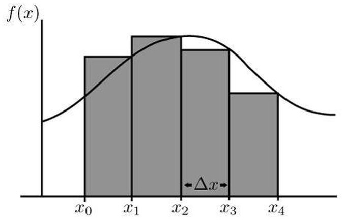
Integrals allow us to calculate the area under a function’s curve. As an example, we’ll calculate the area of the function $f(x) = x$ in the interval $[0, 2]$ . Recall that the area of a rectangle with size $w$ by $h$ is $w \cdot h$ . Our approach will be to construct many smaller rectangles and sum their area.

We start with the case $n = 2$ – two rectangles. We have the data points $x = (1, 2)$ , which give us two rectangles with width and height $(1, f(1))$ and $(1, f(2))$ respectively – note the width is constant because the spaced interval is distributed evenly. To sum the area of this spaced interval, we just sum $1 \cdot f(1) + 1 \cdot f(2) = 3$ . But note that there’s an error, since the rectangles do not cover the whole area. The main idea is the more rectangles, the less the error and the closer we get to the actual value.

Proceed with case $n = 4$ . We have the data points $x = (0.5, 1, 1.5, 2)$ . Since we have four elements, in the range $[0, 2]$ each element has width of $\frac{2 - 0}{4} = 0.5$ . The result is $0.5 [ f(0.5) + f(1) + f(1.5) + f(2) ] = 2.5$ .

Having looked at these cases gives an idea to generalize. First, note the differences of the points in $x$ – when $n = 2$ , the difference between any consecutive points in $x$ is 1, and when $n = 4$ , the difference is $0.5$ . Generalizing for $n$ , the difference between $x_i$ and $x_{i+1}$ will be $\frac{b-a}{n}$ . Also, generalizing the summation gives $\sum_{i=0}^n f(x_i) \cdot \Delta x_i$ , and since we only consider evenly spaced intervals we have $\Delta x_i = \Delta x$ , for all $i$ . This is called a Riemann sum and defines the integral $\int _{a}^{b}f(x)\,\Delta x=\lim_{\Delta x \to 0}\sum_{i=0}^{n}f(x_{i})\Delta x$ , where $\Delta x = \frac{b - a}{n}$ . Also, since $a$ is the starting point, that gives $x_i = a + i \cdot \frac{b-a}{n}$ .

Going back to the example, to find the interval for $f(x) = x$ , we need to calculate $\sum_{i=0}^{n}f(x_{i}) \frac{b - a}{n} = \frac{b - a}{n} \sum_{i=0}^{n}(a + i \cdot \frac{b-a}{n})$ . From here, we evaluate the inner sum $\sum_{i=0}^{n}(a + i \cdot \frac{b-a}{n}) = (n+1)a + \frac{(b - a)(n+1)}{2}$ . Plugging back in gives $(b - a + \frac{b}{n} - \frac{a}{n}) (a + \frac{b - a}{2})$ .

Now we can take the limit of this as $n \to \infty$ . Note that $\lim_{n \to \infty} \frac{a}{n} = 0$ so we have $(b - a)(a + \frac{b-a}{2})$ , which finally gives $\frac{b^2 - a^2}{2}$ . This represents the sum of the area $[a, b]$ under the curve of the function $f(x) = x$ .