Per Wikipedia, an algebraic data type is a kind of composite type, i.e., a type formed by combining other types.
Haskell’s algebraic data types are named such since they correspond to an initial algebra in category theory, giving us some laws, some operations and some symbols to manipulate. — Don Stewart
In Mathematics, there are many curves. From a constant curve , to a linear one , to a quadratic one to …, you name it.
Now, imagine that there is a huge data set with some points (think ordered pairs for simplicity), but not all points are defined. Essentially, machine learning is all about coming up with a curve (based on a chosen model) by filling gaps.
Once we agree on the model we want to use (curve we want to represent), we start with some basic equation and then tweak its parameters until it perfectly matches the data set points. This process of tweaking (optimization) is called “learning”. To optimize, we associate a cost function (the error or delta between the values produced by the equation and the data set) and we need to find for which parameters this cost is minimal.
Gradient descent is one algorithm for finding the minimum of a function, and as such it represents the “learning” part in machine learning. I found this video by StatQuest, along with this video by 3Blue1Brown to be super simple explaining these concepts, and naturally, this article will be mostly based on them.
In this article I will assume some basic set theory, and also derivatives. Further, through example, we will:
I’ve almost finished reading Paul Halmos’ Naive Set Theory. The book is highly technical, therefore it may not be suitable for everyone. I wanted to dig deeper into the technicalities, so that’s the main reason I chose to work through it.
I recommend reading Daniel Velleman’s How To Prove It before tackling this one. How To Prove It is a book about mathematical proofs, but it involves proving properties about sets so you learn both proofs and sets on the way.
Here’s a quick summary of my thoughts on the book and set theory in general.
Introduction
What is a set? A set is a collection of objects. That’s all it is! As simple as that sounds, sets are very important in mathematics. This simplicity is what sparked interest for me.
In fact, (almost) all of mathematics is built upon sets! Set Theory is one of the widely accepted foundations of mathematics. There are also some other theories, but we won’t get into that.
Different mathematical ideas usually need an apparatus to be described. Very often this apparatus is Set Theory.
Examples
Example 1: Consider Probability Theory as a branch of mathematics. To represent a sample space of, for example a dice roll, we usually say . So is a set which contains all the possible outcomes. Rolling an even number is represented by some other set, , where but also note that . There’s a relation between and , and this relation is “subset”, as we have observed. Relations needn’t necessarily be always a subset, but we digress a little. What’s the probability to roll an even number, given the sample space? It’s simply . We just used set theory to calculate the probability of rolling an even number of a 6-sided dice!
If you don’t quite understand the notation in the previous paragraph, don’t worry. It’s really simple, and I have already covered it in a previous post, Abstractions with Set Theory.
Example 2: So Probability was one example, but it goes farther than that. Turing Machines (the computation model that your computer/phone/etc uses) can also be described through set theory. Any computation can be represented through sets, which is really awesome.
Example 3: Another interesting example is natural numbers. They can be represented as: , i.e. the empty set, i.e. a set containing the empty set, , well, you get the idea 😀
Example 4: As we noted earlier, there was a relation between two sets, namely the “subset” relation. Relations can be generalized further, and are used to describe some shared property between objects. For example, may be a valid relation on some set, for example, the natural numbers.
Example 5: Abstraction goes further with Algebraic Structures. For example, a Magma represents a set together with some binary operation (it can be anything!). An example, natural numbers with operation plus makes a Magma.
Conclusion
As you can see, there are too many abstractions! What’s the point in generalizing all of this and introducing all these weird names like Magma, etc? Well, it’s similar to what we do with code. Think about how we generalize some calculations in a large software project and we put them in a function with its own name. We don’t care about the details, we only want to look at it and use it from a different abstraction level. This function has its own properties and behavior which can be observed while we code (e.g. it accepts some specific arguments, or returns either an array or int, etc). Same with mathematics!
Recursion Theorem
Meta: As I mentioned, this book is highly technical. Note this is a 100-page book and I spent almost a year on it – on and off. The thing is, you don’t read it like a storybook. Think of it more like a Sudoku puzzles book. When I’m in the mood, I sit down and “solve” some puzzles. Sometimes, even for myself, some of the technical explanations are hard to understand. But I don’t give up – I re-read them a lot of times. When it clicks, I get a very good feeling. Like when you learn a new trick. It’s a very similar feeling to programming. Try to think of some task that you worked on and you learned a new cool trick. It feels good, and you can’t wait to apply this trick again and again until it gets boring. 🙂
So we can conclude that Set Theory is a really powerful apparatus. I hope these examples sparked some interest for you too!
We’re in the process of renovating our house with my wife.
We have a bunch of “engineers” working on it: electricians, plumbers, wall painters. These guys have direct contact with the customers. What they are working on will be immediately visible to the customer. They must be thinking about the customer all the time, and satisfy their needs. There is no management, customer support, release dates in between (I’m sure there is for larger objects). What they are doing is visible at the spot and they must make sure it looks right, otherwise the customer will be mad.
This sounds very similar to what freelancing software engineers are doing. On the other hand, software engineers that work at big companies have huge layers before they reach the customers. As a consequence, most of them even rarely think about their customers at all.
Lately I’ve been thinking about our customers more and more. What we are building as software engineers are decisions that were discussed with other smart people at meetings, etc. But I think there is still value in constantly asking yourself: “what will the customer think about this?”, “what will their reaction be on what I’m building right now”, etc.
Do you ever think about your customers, or only your code like most of us? 🙂
Lately I’ve been thinking about this: What do we get if we change lambda calculus’s abstraction from (λx.M) to (λN.M), where M and N are lambda terms, and x is a variable?
type VarName = String

data Term =
    TmVar VarName
    | TmAbs Term Term
    | TmApp Term Term deriving (Eq, Show)
With the new list of inference rules:
Name
Rule
E-App1
E-App2
E-App3
E-AppAbs
So the evaluator looks something like:
eval : Term -> Term
eval (TmApp (TmAbs (TmVar x) t12) v2)      = subst x t12 v2 -- E-AppAbs
eval (TmApp (TmAbs v1@(TmAbs _ _) t12) t2) = let t2' = eval t2 in let v1' = eval (TmApp v1 t2') in TmAbs v1' t12 -- E-App3
eval (TmApp v1@(TmAbs _ _) t2)             = let t2' = eval t2 in TmApp v1 t2' -- E-App2
eval (TmApp t1 t2)                         = let t1' = eval t1 in TmApp t1' t2 -- E-App1
eval (TmVar x)                             = TmVar x -- E-Var
eval x                                     = error ("No rule applies: " ++ show x)
subst is the same as in the previous post.
So with this system we could “control” the “arguments” in the abstraction through application.
We could represent λx.x and λy.x through a single abstraction, i.e. (λ(λx . x) . x) so we get to either pass x or y to it:
Main> let f1 = TmAbs (TmVar "x") (TmVar "x")
Main> let f2 = TmAbs (TmVar "y") (TmVar "x")
Main> let f3 = TmAbs (TmAbs (TmVar "x") (TmVar "x")) (TmVar "x")
Main> eval (TmApp f3 (TmVar "x")) == f1
True
Main> eval (TmApp f3 (TmVar "y")) == f2
True
Is this useful or not? I didn’t know 🙂 so as always I referred to ##dependent@freenode and learned a bunch of new stuff:
 <pgiarrusso> I suspect many metaprogramming facilities would allow generating `𝜆 foo. x` by picking `foo`, but I don't see any reason to support this specifically
 <pgiarrusso> to be sure, I'm not necessarily saying "there is no point"
 <pgiarrusso> also, for your example, it seems `if foo then λx.x else λy.x` would work as well
 <pgiarrusso> my best answer is, when you write a function, you want to know what are the function params, to refer to them
Some stuff on papers:
 <pgiarrusso> *now*, I'm sure that strange variants of LC exist which do make sense but look surprising
 <pgiarrusso> but I think people usually start from something that is (1) useful but (2) hard, and then build a formal system to support that
 <pgiarrusso> s/people/researchers/
 <bor0> how do they know that it's useful?
 <pgiarrusso> sometimes you do go the opposite way, but that's harder
 <pgiarrusso> bor0: take a PL paper, read the introduction, see the arguments they make
 <bor0> I don't understand how that determines the usefulness of the paper itself?
 <bor0> or the idea even
 <pgiarrusso> bor0: not sure what paper to pick, but http://worrydream.com/refs/Hughes-WhyFunctionalProgrammingMatters.pdf might be an example
 <pgiarrusso> lots of that paper is an argument that lazy evaluation is interesting and useful
 <pgiarrusso> it does not *prove* that it's useful, as that's not something you can prove
 <pgiarrusso> but that paper (and many others) show something that is hard to do, arguably desirable, and give a "better" way of doing it
Bonus 🙂
 <mietek> bor0: <gallais> Someone was talking about a lambda calculus with full terms instead of mere variables in binding position IIRC
 <mietek> bor0: <gallais> I just came across this work: https://academic.oup.com/jigpal/article/26/2/203/4781665
 <bor0> wow thanks mietek!
 <bor0> interesting how when humans think about a certain topic they almost always have overlapping ideas
 <bor0> (:philosoraptor: it just confirms Wadler's statement that mathematics is discovered, not invented, I guess)
 <bor0> but I am happy that I had thought of that, even if for 2 years late (article was published in 2017)
Update: Thanks to /u/__fmease__ for noticing an error in the E-App3 LaTeX rule.
 , to a linear one
  , to a quadratic one
  to …, you name it.
 . So
. So  is a set which contains all the possible outcomes. Rolling an even number is represented by some other set,
  , where
  but also note that
  . There’s a relation between
  . We just used set theory to calculate the probability of rolling an even number of a 6-sided dice!
 , i.e. the empty set,
  i.e. a set containing the empty set,
  , well, you get the idea 😀
 may be a valid relation on some set, for example, the natural numbers.
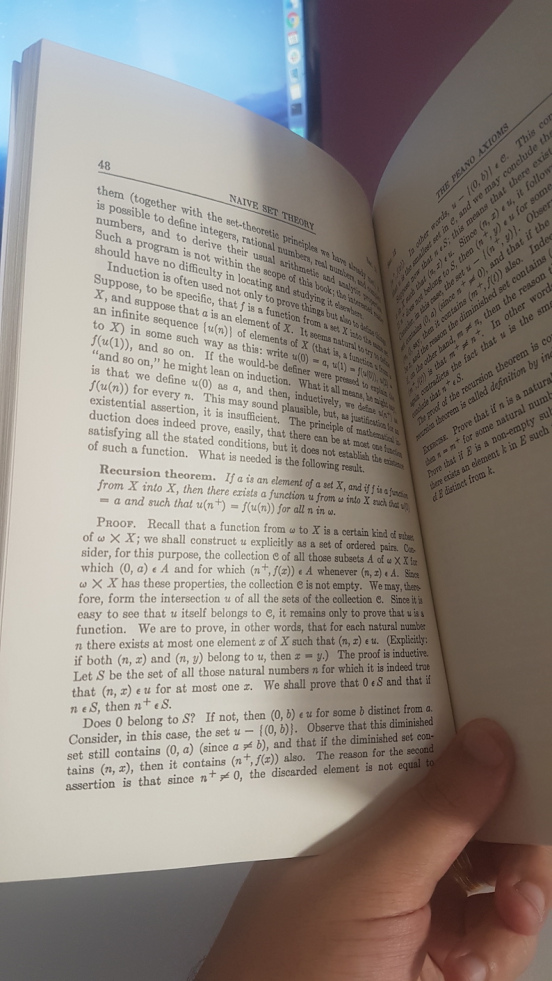


![(\lambda x.t_{12})v_2 \to [x \mapsto v_2]t_{12}](https://s0.wp.com/latex.php?latex=%28%5Clambda+x.t_%7B12%7D%29v_2+%5Cto+%5Bx+%5Cmapsto+v_2%5Dt_%7B12%7D&bg=ffffff&fg=000000&s=0&c=20201002)
