Grand Meetup is an event here at Automattic where the whole company gathers once a year to do classes, projects, or just hack around ideas in general.
This year it was held in Whistler, BC, Canada.
Working remotely with strangers and meeting them in person was a bit weird and overwhelming in the beginning.
However, I had already met my team during a team meetup in Vienna, so hanging out with them during the GM was more relaxing 🙂
I also met Matt!
Then, besides meeting all of these nice folks, I also played my first D&D game ever! My character was a Human Wizard (named Matt :D) and we slayed the dragon!
The food at the hotels was really good!
The village had some really nice views! We went for some souvenir shopping.
Then, for the closing party we had some arcades!
Also, my team Woo rocked the stage 😀
Some stats: before the GM I had met 1% of all Automatticians. Now that has moved up to around 20%. With that, my objective of meeting all the folks that I have interacted or worked with was completed!
So a few words about the company: Automattic is about transparency, passion, freedom, impact, people, differences. If you care about these things, Automattic is hiring and you can apply.
During my js ⊂ lisp talk at beerjs, I noticed there were a few questions about recursion and tail call recursion, so with this post I hope to address that.
To start with, let’s define the following methods for creating a pair and getting its values:
An iterative process is characterized by a process whose state is captured with variables and rules how to transform them to the next state.
A recursive process is characterized by a chain of deferred evaluations. Note that a recursive procedure need not always generate a recursive process.
An iterative procedure is a procedure that does not have any references to itself.
A recursive procedure is a procedure that has references to itself.
With this, we see that there are recursive processes, and there are recursive procedures. Combining those, we get the following table:
Process / Procedure
Iterative
Recursive
Iterative
1
2
Recursive
3
4
Now that we’ve classified the combinations, we can discuss their properties and characteristics by examples:
An iterative process with iterative procedure. No recursion is involved, and there is no need for deferred evaluations (since the process is iterative). It can be further optimized using other looping constructs than goto, but we will write it this way to show the similarity with 3.
// Iterative process, iteration (for languages that don't support tail call optimization)
function lengthiter_i( $pair, $acc = 0 ) {
begin:
if ( null === $pair ) {
return $acc;
}        $pair = cdr( $pair );
$acc  = 1 + $acc;
goto begin;
}
A recursive process with iterative procedure. Recursion is involved, but since the procedure is iterative, we will implement it with the help of a list (stack), e.g. to allow for deferred evaluations in some cases:
An iterative process with recursive procedure. Similar to the iterative process with iterative procedure, although differently implemented. May fail on languages that don’t have tail call optimization. Compare this code to 1 to see the similarity (additionally we map the arguments $pair => cdr( $pair ) and $acc => 1 + $acc).
A recursive process with recursive procedure. Similar to the recursive process with iterative procedure, although differently implemented in the way that the stack is implicit by calling the function multiple times, so we don’t need to handle it ourselves. For example:
To reach to here, we first had to work out the point slope formula and then figure out limits. Derivatives are very powerful. This post was inspired by doing gradient descent on artificial neural networks, but I won’t cover that here. Instead we will focus on the very own definition of a derivative.
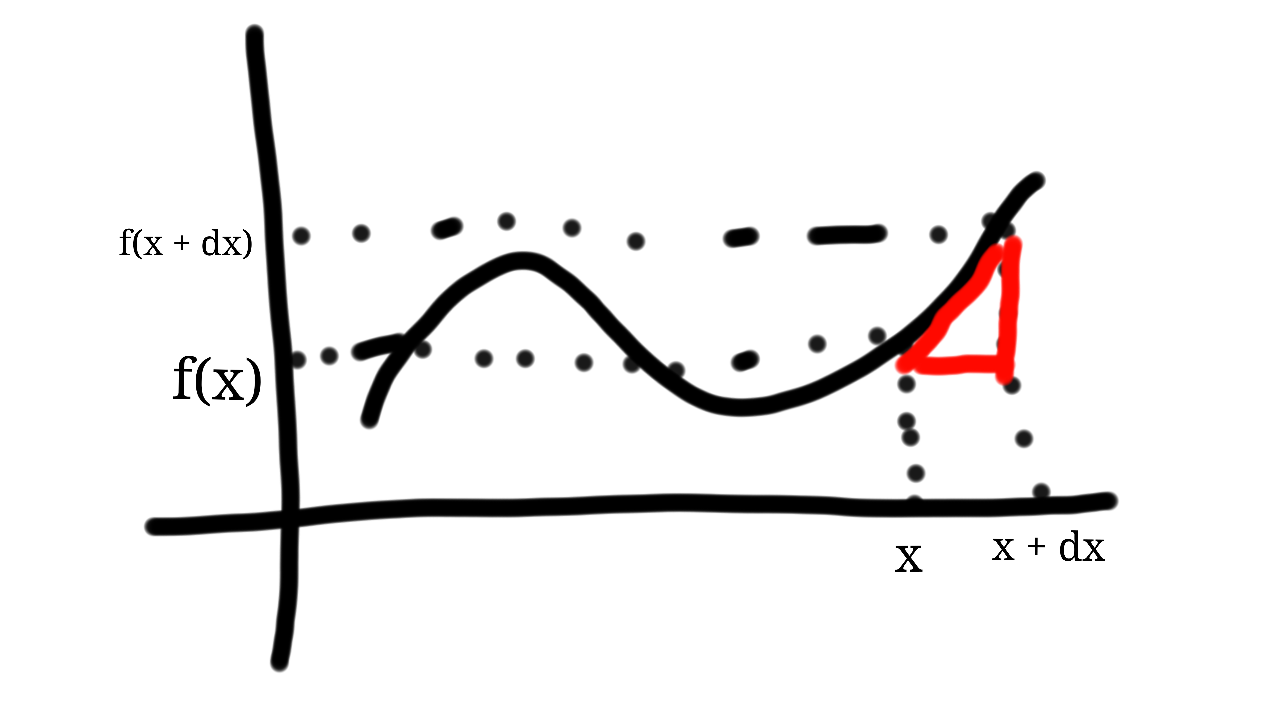
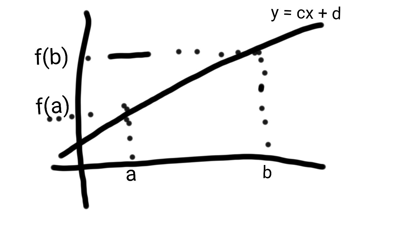
So let’s get started. A secant is a line that goes through 2 points. In the graph below, the points are and .
To derive a formula for this, we can use the point-slope form of a equation of a line: .
Plugging in the values, we get: .
What is interesting about this formula using the secant is that, as we will see, it provides us with a neat approximation at f(x). Let’s define . So now we have: .
The limit as dx approaches 0 for will give us the actual slope (according to the definition of an equation of a line) at x.
So, let’s define . This slope is actually our definition of a derivative. This definition lies at the heart of calculus.
The image below (taken from Wikipedia) demonstrates this for h = dx.
Back to the secant approximation, we now have: . This is an approximation rather than an equivalence because we already calculated the limit for one term but not the rest. As dx -> 0, the approximation -> equivalence.
For example, to calculate the square of 1.5, we let x = 1 and dx = 0.5. Additionally, if then . So . That’s an error of just 0.25 for dx = 0.5. Algebra shows for this particular case the error to be dx^2. For dx = 0.1, the error is just 0.01.
Pretty cool, right?
Here are some of the many applications to understand why derivatives are useful:
We can use the value of the slope to find min/max using gradient descent
We can determine the rate of change given the slope
We can find ranges of monotonicity
We can do neat approximations, as shown
Integrals allow us to calculate the area under a function’s curve. As an example, we’ll calculate the area of the function in the interval . Recall that the area of a rectangle with size by is . Our approach will be to construct many smaller rectangles and sum their area.
We start with the case – two rectangles. We have the data points , which give us two rectangles with width and height and respectively – note the width is constant because the spaced interval is distributed evenly. To sum the area of this spaced interval, we just sum . But note that there’s an error, since the rectangles do not cover the whole area. The main idea is the more rectangles, the less the error and the closer we get to the actual value.
Proceed with case . We have the data points . Since we have four elements, in the range each element has width of . The result is .
Having looked at these cases gives an idea to generalize. First, note the differences of the points in – when , the difference between any consecutive points in is 1, and when , the difference is . Generalizing for , the difference between and will be . Also, generalizing the summation gives , and since we only consider evenly spaced intervals we have , for all . This is called a Riemann sum and defines the integral , where . Also, since is the starting point, that gives .
Going back to the example, to find the interval for , we need to calculate . From here, we evaluate the inner sum . Plugging back in gives .
Now we can take the limit of this as . Note that so we have , which finally gives . This represents the sum of the area under the curve of the function .
This post assumes knowledge in mathematical logic and algebra.
We will stick to sequences for simplicity, but the same reasoning can be extended to functions. For sequences we have one direction: infinity.
Informally, to take the limit of something as it approaches infinity is to determine its eventual value at infinity (even though it may not ever reach it).
As an example, consider the sequence . The first few elements are: 1, 0.5, 0.(3), 0.25, and so on.
Note that is undefined as infinity is not a real number. So here come limits to the rescue.
If we look at its graph, it might look something like this:
We can clearly see a trend that as x -> infinity, 1/x tries to “touch” the horizontal axis, i.e. is equal to 0. We write this as such: .
Formally, to say that , we denote: . Woot.
It looks scary but it’s actually quite simple. Epsilon is a range, N is usually a member that starts to belong in that range, and the absolute value part says that all values after that N belong in this range.
So for all ranges we can find a number such that all elements after that number belong in this range.
Why does this definition work? It’s because when the range is too small, all elements after N belong in it, i.e. the values of the sequence converge to it endlessly.
As an example, let’s prove that . All we need to do is find a way to determine N w.r.t. Epsilon and we are done.
Suppose Epsilon is arbitrary. Let’s try to pick N s.t. .
Let’s see how it looks for : for , we have: . This is obviously true since . So there’s our proof.
This bit combined with the slope point formula form the derivative of a function, which will be covered in the next post.


 and
and  .
.
 .
. .
. . So now we have:
  .
. will give us the actual slope (according to the definition of an equation of a line) at x.
 . This slope is actually our definition of a derivative. This definition lies at the heart of calculus.
 . This is an approximation rather than an equivalence because we already calculated the limit for one term but not the rest. As dx -> 0, the approximation -> equivalence.
 then
then  . So
. So  . That’s an error of just 0.25 for dx = 0.5. Algebra shows for this particular case the error to be dx^2. For dx = 0.1, the error is just 0.01.
 in the interval
 ![[0, 2]](https://s0.wp.com/latex.php?latex=%5B0%2C+2%5D&bg=ffffff&fg=000000&s=0&c=20201002) . Recall that the area of a rectangle with size
. Recall that the area of a rectangle with size  by
by  is
is  . Our approach will be to construct many smaller rectangles and sum their area.
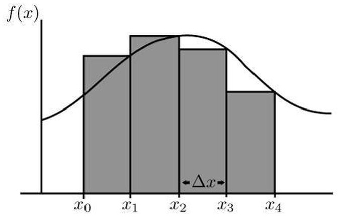
 – two rectangles. We have the data points
  , which give us two rectangles with width and height
  and
and  respectively – note the width is constant because the spaced interval is distributed evenly. To sum the area of this spaced interval, we just sum
  . But note that there’s an error, since the rectangles do not cover the whole area. The main idea is the more rectangles, the less the error and the closer we get to the actual value.
 . We have the data points
  . Since we have four elements, in the range
  . The result is
 ![0.5 [ f(0.5) + f(1) + f(1.5) + f(2) ] = 2.5](https://s0.wp.com/latex.php?latex=0.5+%5B+f%280.5%29+%2B+f%281%29+%2B+f%281.5%29+%2B+f%282%29+%5D+%3D+2.5&bg=ffffff&fg=000000&s=0&c=20201002) .
. – when
  . Generalizing for
  , the difference between
  and
and  will be
  . Also, generalizing the summation gives
  , and since we only consider evenly spaced intervals we have
  , for all
  . This is called a Riemann sum and defines the integral
  , where
  . Also, since
  is the starting point, that gives
  .
. . From here, we evaluate the inner sum
  . Plugging back in gives
  .
. . Note that
  so we have
  , which finally gives
  . This represents the sum of the area
 ![[a, b]](https://s0.wp.com/latex.php?latex=%5Ba%2C+b%5D&bg=ffffff&fg=000000&s=0&c=20201002) under the curve of the function
under the curve of the function  . The first few elements are: 1, 0.5, 0.(3), 0.25, and so on.
 is undefined as infinity is not a real number. So here come limits to the rescue.
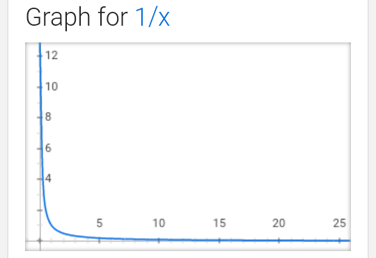
 .
. , we denote:
  . Woot.
 .
. : for
: for  , we have:
  . This is obviously true since
  . So there’s our proof.
 , this line passes through the point
  .
. .
.


 .
.