Curry–Howard correspondence

For most of my schooling (basic school, high school), I’ve had a private math teacher thanks to my parents. I believe this has shaped my career path for the better.

I’ve always wanted to be a programmer, and I used to be interested in nothing else. Now I am lucky for the past years to be doing exactly what I’ve always wanted, and that is programming.

Back in basic school, I remember one thing that one of my math teachers kept reminding me: “Study math, it is very closely related to programming”. Now I think I really understand what that statement means.

In any case, I’ve recently started digging into Lean Theorem Prover by Microsoft Research. Having some Haskell experience, and experience with mathematical proofs, the tutorial is mostly easy to follow.

I don’t have much experience with type theory, but I do know some stuff about types from playing with Haskell. I’ve heard about the Curry-Howard correspondence a bunch of times, and it kind of made sense, but I haven’t really understood it in depth. So, by following the Lean tutorial, I got to get introduced to it.

An excerpt from Wikipedia:

In programming language theory and proof theory, the Curry–Howard correspondence (also known as the Curry–Howard isomorphism or equivalence, or the proofs-as-programs and propositions- or formulae-as-types interpretation) is the direct relationship between computer programs and mathematical proofs.

In simpler words, a proof is a program, and the formula it proves is the type for the program.

Now as an example, consider your neat function of swapping 2 values of a product type:

swap :: (a, b) -> (b, a)
swap (a, b) = (b, a)

What the Curry-Howard correspondence says is that this has an equivalent form of a mathematical proof.

Although it may not be immediately obvious, think about the following proof:
Given P and Q, prove that Q and P.
What you do next is use and-introduction and and-elimination to prove this.

How does this proof relate to the swap code above? To answer that, we can now consider these theorems within Lean:

variables p q : Prop
theorem and_comm : p ∧ q → q ∧ p := fun hpq, and.intro (and.elim_right hpq) (and.elim_left hpq)

variables a b : Type
theorem swap (hab : prod a b) : (prod b a) := prod.mk hab.2 hab.1

Lean is so awesome it has this #check command that can tell us the complete types:

#check and_comm -- and_comm : ∀ (p q : Prop), p ∧ q → q ∧ p
#check swap     -- swap     : Π (a b : Type), a × b → b × a

Now the shapes are apparent.

We now see the following:

and.intro is equivalent to prod.mk (making a product)
and.elim_left is equivalent to the first element of the product type
and.elim_right is equivalent to the second element of the product type
forall is equivalent to the dependent type pi-type
A dependent type is a type whose definition depends on parameters. For example, consider the polymorphic type List a. This type depends on the value of a. So List Int is a well defined type, or List Bool is another example.

More formally, if we’re given A : Type and B : A -> Type, then B is a set of types over A.
That is, B contains all types B a for each a : A.
We denote it as Pi a : A, B a.

As a conclusion, it’s interesting how logical AND being commutative is isomorphic to a product type swap function, right? 🙂

Induction with Coq

To get ourselves introduced to the induction tactic, we’ll start by showing that 0 is a right identity for the naturals under addition, i.e. $\forall n \in \mathbb{N}, n + 0 = n$ .

The definition of addition is: $n = 0 + n, S(m) + n = S(m + n)$ .

Mathematically, we start with induction on n.

We have $0 + 0 = 0$ for the base case, which is true (based on definition of add).
For the inductive step, we assume that $n + 0 = n$ , and try to prove that $S n + 0 = S n$ .
We can rewrite our goal by using the definition of add, where we have $S n + 0 = S (n + 0)$ .
Now using the hypothesis we have $S (n + 0) = S n$ , which is what we needed to show.

Programmatically, we have:

Compute 2+3. (* Test to see what's 2 plus 3 *)

Theorem zero_identity_on_addition : (forall n:nat, n + 0 = n).
Proof.
  intros n.
  induction n.     (* Use induction on n *)
  (* Base case *)
    simpl.         (* Simplify 0 + 0 = 0 to 0 = 0 *)
    exact eq_refl. (* Which is exactly reflexivity *)
  (* Inductive step *)
  simpl.           (* At this point we have S n + 0 = S n, in other words n + 1 + 0 = n + 1 *)
                   (* Simplify to get (n + 0) + 1 = n + 1 *)
  rewrite IHn.     (* Use the hypothesis to rewrite (n + 0) to n *)
  exact eq_refl.   (* n + 1 = n + 1 is proven by reflexivity *)
Qed.

Neat, right?

Our second example is more complex. We will:
1. Define a recursive function, fact.
2. Prove that $fact(3) = 6$ .
3. Introduce and prove a lemma to be used for our proof.
4. Prove that $fact(n) > 0$ .

Mathematically:

$fact(n) = \left\{ \begin{array}{ll} 1 & \mbox{if } n = 0 \\ n * fact(n - 1) & \mbox otherwise \end{array} \right.$
To show what fact(3) is, we go by definitions: $3 * fact(2) = 3 * 2 * fact(1) = 3 * 2 * 1 * fact(0) = 6$ .
To prove $x > 0 \implies x + y > 0$ , which is the lemma we’ll use in our Coq proof, note we have as givens $x > 0, y \ge 0$ (since $y \in \mathbb{N}$ ).

From here, we have two cases:
$\begin{cases} y = 0: x + y = x + 0 = x > 0 \\ y > 0: x + y > 0 + x = x > 0 \end{cases}$

By transitivity on $(>, \mathbb{N})$ for the second case, combined with the first case, we can conclude that $x + y > 0$ .
To prove that $fact(n) > 0$ for $n \ge 0$ , we use induction on n.

Base case: $n = 0: fact(0) = 1 > 0$ , which is true.
Inductive step: Assume $fact(k) > 0$ for some $n = k$ . Note that $n \ge 0 \implies k + 1 > 0$ , so we’re good to multiply with a positive number.

Multiply both sides by k + 1 to get $(k + 1) * fact(k) = fact(k + 1) > 0$ , which is what we needed to show.

Thus $fact(n) > 0$ in general.

Now for the programming part.

The recursive definition:

(* If we try to use Definition, we get fact is not defined *)
(* Coq provides a special syntax Fixpoint for recursion *)
Fixpoint fact (n:nat) : nat :=
  match n with
    | S n => S n * fact n
    | 0 => 1
end.

Evaluate and prove $fact(3) = 6$

Compute (fact 3).
 
Theorem fact_3_eq_6 : (fact 3 = 6).
Proof.
  simpl.           (* Evaluate fact 3 = 6 *)
  exact eq_refl.   (* 6 = 6 is exactly reflexivity *)
Qed.

We start our lemma as follows:

Require Import Coq.Arith.Plus.

Lemma x_plus_y_gt_0 : (forall x y : nat, x > 0 -> x + y > 0).
Proof.
  intros x y.
  intros x_gt_0.
  unfold gt.           (* Convert x + y > 0 to 0 < x + y *) 
  unfold gt in x_gt_0. (* Convert x_gt_0 : x > 0 to x_gt_0 : 0 < x *)
  (* We have that Theorem lt_plus_trans n m p : n < m -> n < m + p *)
  (* So we feed 0, x, y to match the arguments, and additionally pass x_gt_0 to match the n < m part *)
  exact (lt_plus_trans 0 x y x_gt_0).
Qed.

Nothing new going on here. But, we can try to be smart, and try to rewrite the lemma as:

Require Import Omega.

Lemma x_plus_y_gt_0 : (forall x y : nat, x > 0 -> x + y > 0).
Proof.
  intros x y.
  omega.
Qed.

The new thing we can notice here is the usage of the omega tactic.

This tactic is an automatic decision procedure for Presburger arithmetic, i.e. it will solve any arithmetic-based proof goal that it understands (and that is true). But note e.g. that it doesn’t understand multiplication.

The actual proof

Theorem fact_gt_0 : (forall n : nat, fact n > 0).
Proof.
  intros n.
  induction n.
  (* Base case *)
    simpl.          (* At this point we have fact 0 > 0, simplify to get 1 > 0 *)
    exact (le_n 1). (* This is exactly 1 > 0 *)
  (* Inductive step *)
    simpl.          (* Simplify to convert fact(n + 1) > 0 to fact n + n * fact n > 0 *)
                    (* Which is exactly our lemma defined above *)
                    (* We also have IHn : fact n > 0 *)
    (* Feed (fact n), (n * fact n) into x_plus_y_gt_0, and IHn as well for the x > 0 part *)
    exact (x_plus_y_gt_0 (fact n) (n * fact n) IHn).
Qed.

Thus, the complete program:

Require Import Omega.

(* If we try to use Definition, we get fact is not defined *)
(* Coq provides a special syntax Fixpoint for recursion *)
Fixpoint fact (n:nat) : nat :=
  match n with
    | S n => S n * fact n
    | 0 => 1
end.

Compute (fact 3).

Theorem fact_3_eq_6 : (fact 3 = 6).
Proof.
  simpl.           (* Evaluate fact 3 = 6 *)
  exact eq_refl.   (* 6 = 6 is exactly reflexivity *)
Qed.

Lemma x_plus_y_gt_0 : (forall x y : nat, x > 0 -> x + y > 0).
Proof.
  intros x y.
  omega.
Qed.

Theorem fact_gt_0 : (forall n : nat, fact n > 0).
Proof.
  intros n.
  induction n.
  (* Base case *)
    simpl.          (* At this point we have fact 0 > 0, simplify to get 1 > 0 *)
    exact (le_n 1). (* This is exactly 1 > 0 *)
  (* Inductive step *)
    simpl.          (* Simplify to convert fact(n + 1) > 0 to fact n + n * fact n > 0 *)
                    (* Which is exactly our lemma defined above *)
                    (* We also have IHn : fact n > 0 *)
    (* Feed (fact n), (n * fact n) into x_plus_y_gt_0, and IHn as well for the x > 0 part *)
    exact (x_plus_y_gt_0 (fact n) (n * fact n) IHn).
Qed.

As a conclusion from the examples above, we can say that Coq with its type mechanism provides a neat way for us to reason about properties of our programs.

More proofs and tactics with Coq

If you look at the Tactics index, you will find many useful tactics to use in attempt to prove what you’re trying to prove.

One interesting example I’ve found is the auto tactic.

This tactic implements a Prolog-like resolution procedure to solve the current goal. So let’s try it and see how we can use it:

Goal (5 > 4).
  auto.       (* This magical command tries to prove stuff automatically *)
  Show Proof. (* And show us how it did it *)
Qed.

It’s proven 5 > 4 very easily, and with Show Proof we can additionally see how it did that. We see it used le_n 5, so now we can rewrite our proof:

Goal (5 > 4).
  exact (le_n 5).
Qed.

We could also dig into le_n to see what it actually does.

In our next example we’ll have a look at the case tactic (we’ve already used destruct before):

Require Import Bool.

Notation "x && y" := (andb x y).

Theorem x_and_true : (forall x : bool, x && true = x).
Proof.
  intros x.
  case x. (* Case analysis on x *)
  (* Handle the case where x is true *)
    simpl.       (* Simplify true && true *)
    reflexivity. (* true = true is proven by reflexivity *)
  (* Handle the case where x is false *)
    simpl.       (* Simplify false && true *)
    reflexivity. (* false = false is proven by reflexivity *)
Qed.

As you can see we’re relying on the Bool package and its function andb, but for simplicity we wrote an alias for it (&&) to use as infix operator.

We can check how Bool is defined, and if we do that we’ll see it has 2 options (true, false) and we’re ready to use case.

When we say case on something of type bool, it will go through the cases in order, so it starts with true, and once we prove that case it will proceed with false.

Our last (and most complex) example is where we introduce ourselves to the unfold tactic, and also rely on external proofs:

Require Import PeanoNat.

Theorem x_gte_5_x_gt_4 : (forall x : nat, x = 5 \/ x > 5 -> x > 4).
Proof.
  intros x.
  intros x_gte_5.
  case x_gte_5.
  (* Handle case x = 5 *)
    intros x_eq_5.  (* At this point we have x = 5 and x > 4 *)
    rewrite x_eq_5. (* Rewrite x > 4 with x = 5 to get 5 > 4 *)
    exact (le_n 5). (* Check le_n in Coq library, 5 > 4 is exactly that *)
  (* Handle case x > 5 *)
    (* Coq's ">" (gt) is defined in terms of "<" (lt), so we unfold to convert *)
    unfold gt.      (* At this point we have 5 < x -> 4 < x *)
    (* Check lt_succ_l in Coq library, 5 < m -> 4 < m is exactly that (which is why we used unfold) *)
    exact (Nat.lt_succ_l 4 x).
Qed.

In our next post we’ll be looking at the induction tactic, as well as some examples for it.

My first proofs in Coq

Lately I’ve been spending some time working on Mike Nahas’s tutorial, for the Coq theorem prover.

Here’s a quick summary of what I’ve learned:

Coq is structured into 3 languages:
– Vernacular language – manages definitions, e.g. commands “Theorem”, “Proof”, “Qed”.
– Tactics language – the commands we use to do the proofs themselves, e.g. intros, pose, destruct, exact, etc.
– Gallina language – where we specify what we want to prove, e.g. (forall A B : Prop, A /\ B -> B).

Here’s the first proof I’ve managed to do myself:

Theorem my_first_proof : (forall A B : Prop, A /\ B -> B).
Proof.
  intros A B.     (* These are the Props *)
  intros A_and_B. (* This is A and B from the Gallina definition above *)
  destruct A_and_B as [proof_A proof_B].
  (* At this point we've destructed A_and_B innto proof_A : A and proof_B : B *)
  exact proof_B.  (* This is exactly proof_B *)
Qed.

And here’s how that looks in CoqIDE:

Here’s my second proof, which uses the pose tactic to do a rename:

Theorem my_second_proof : (forall A B : Prop, A -> (A -> B) -> B).
Proof.
  intros A B.     (* These are the Props *)
  intros proof_A. (* This is the proof of A *)
  intros A_imp_B. (* This is A -> B)
  pose (proof_B := A_imp_B proof_A).
  (* At this point, proof_B is actually the combination of A -> B and A, which is B *)
  exact proof_B.  (* And is exactly what we needed. We could've also just do  exact (A_imp_B proof_A). instead *)
Qed.

Proving conditionals:

Theorem my_third_proof : (forall A B : Prop, A -> A \/ B).
Proof.
  intros A B.
  intros proof_A.
  pose (proof_A_or_B := or_introl proof_A : A \/ B).
  exact proof_A_or_B.
Qed.

We had to use the built-in or_introl proof for the type “or”. Note that “Inductive” allows us to create a new type. In addition, we had to explicitly set the type of the proof_A_or_B.

Finally, let’s define our week days, have a function that calculates the next day and prove that after Monday comes Tuesday:

Inductive Day : Set :=
  | Mon : Day
  | Tue : Day
  | Wed : Day
  | Thu : Day
  | Fri : Day
  | Sat : Day
  | Sun : Day.

Definition Next (day : Day) : Day :=
  match day with
    | Mon => Tue
    | Tue => Wed
    | Wed => Thu
    | Thu => Fri
    | Fri => Sat
    | Sat => Sun
    | Sun => Mon
  end.

Eval compute in Next Mon.

Theorem after_monday_simple : ((Next Mon) = Tue).
Proof.
  simpl.         (* Evaluate (Next Mon) which is Tue as we've seen above *)
  exact eq_refl. (* This is exactly reflexivity on equality. *)

  (* Could also just use reflexivity here, but note that reflexivity does simpl implicitly *)
  (* reflexivity. (* Tue = Tue is proven by reflexivity *) *)
Qed.

Theorem after_monday : (forall A : Day, A = Mon -> Next A = Tue).
Proof.
  intros A.
  intros A_eq_Mon.
  rewrite A_eq_Mon. (* Instead of trying to prove Next A = Tue, try to prove Next Mon = Tue *)
  simpl.
  constructor.      (* Since reflexivity does simpl implicitly, it makes more sense to use this instead *)
Qed.

And some interesting discussion on #coq @ freenode:

 <bor0> how many tactic commands are there like in total? 😀
 <johnw> 191 in Coq 8.5
 <bor0> wow, that's a lot. and I've only got introduced to about 10 or so
 <johnw> you don't need to know all of them, by any means
 <johnw> some are the more basic tactics from which other tactics are built up
 <johnw> think of it like a standard tactic library
 <johnw> that's the beauty of all this: almost everything is just about types and finding inhabitants of types

Fun stuff, right? 🙂

Deriving derivative and integral

To reach to here, we first had to work out the point slope formula and then figure out limits. Derivatives are very powerful. This post was inspired by doing gradient descent on artificial neural networks, but I won’t cover that here. Instead we will focus on the very own definition of a derivative.

So let’s get started. A secant is a line that goes through 2 points. In the graph below, the points are $A = (x, f(x))$ and $A' = (x + dx, f(x + dx))$ .

To derive a formula for this, we can use the point-slope form of a equation of a line: $y - y_0 = \frac {y_1 - y_0} {x_1 - x_0} (x - x_0)$ .

Plugging in the values, we get: $f(x) - f(x + dx) = - \frac {f(x + dx) - f(x)} {dx} (dx)$ .

What is interesting about this formula using the secant is that, as we will see, it provides us with a neat approximation at f(x).
Let’s define $f_{new}(x, dx) = \frac {f(x + dx) - f(x)} {dx}$ . So now we have: $f(x + dx) = f(x) + f_{new}(x, dx) (dx)$ .

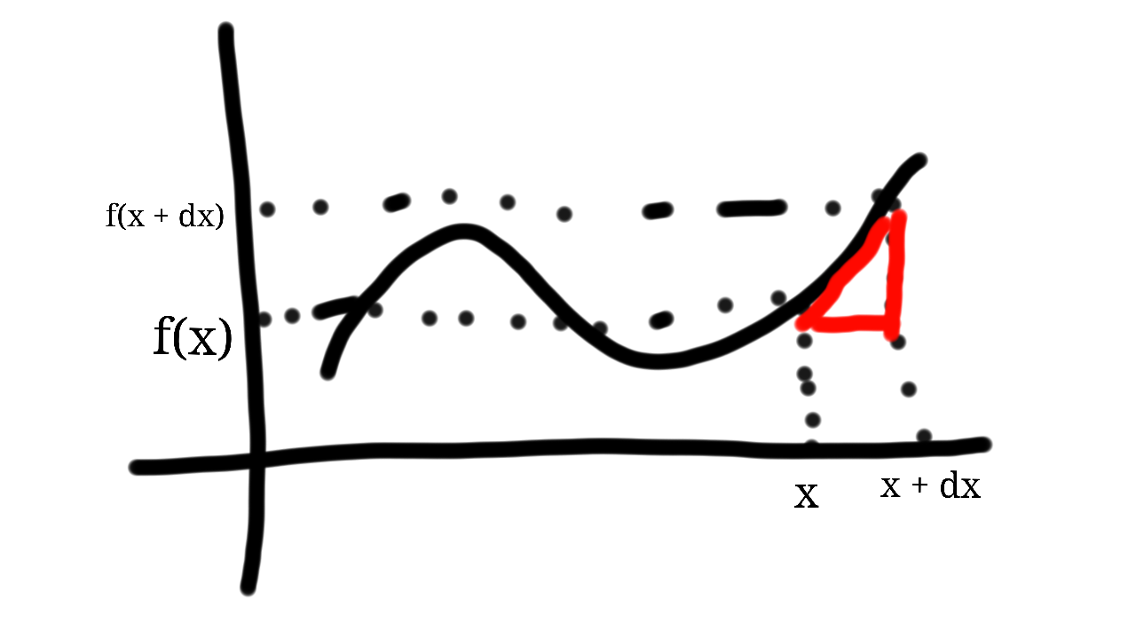
The limit as dx approaches 0 for $f_{new}$ will give us the actual slope (according to the definition of an equation of a line) at x.

So, let’s define $\lim_{dx \to 0} f_{new}(x, dx) = f'(x)$ . This slope is actually our definition of a derivative. This definition lies at the heart of calculus.

The image below (taken from Wikipedia) demonstrates this for h = dx.

Back to the secant approximation, we now have: $f(x + dx) \approx f(x) + f'(x) (dx)$ . This is an approximation rather than an equivalence because we already calculated the limit for one term but not the rest. As dx -> 0, the approximation -> equivalence.

For example, to calculate the square of 1.5, we let x = 1 and dx = 0.5. Additionally, if $f(x) = x^2$ then $f'(x) = x*2$ . So $f(1 + 0.5) = f(x + dx) \approx f(1) + f'(1) 0.5 = 1 + 2 * 1 * 0.5 = 2$ . That’s an error of just 0.25 for dx = 0.5. Algebra shows for this particular case the error to be dx^2. For dx = 0.1, the error is just 0.01.

Pretty cool, right?

Here are some of the many applications to understand why derivatives are useful:

We can use the value of the slope to find min/max using gradient descent
We can determine the rate of change given the slope
We can find ranges of monotonicity
We can do neat approximations, as shown

Integrals allow us to calculate the area under a function’s curve. As an example, we’ll calculate the area of the function $f(x) = x$ in the interval $[0, 2]$ . Recall that the area of a rectangle with size $w$ by $h$ is $w \cdot h$ . Our approach will be to construct many smaller rectangles and sum their area.

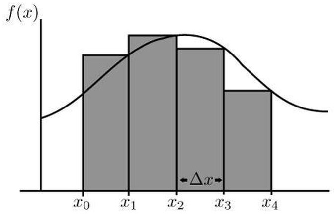
We start with the case $n = 2$ – two rectangles. We have the data points $x = (1, 2)$ , which give us two rectangles with width and height $(1, f(1))$ and $(1, f(2))$ respectively – note the width is constant because the spaced interval is distributed evenly. To sum the area of this spaced interval, we just sum $1 \cdot f(1) + 1 \cdot f(2) = 3$ . But note that there’s an error, since the rectangles do not cover the whole area. The main idea is the more rectangles, the less the error and the closer we get to the actual value.

Proceed with case $n = 4$ . We have the data points $x = (0.5, 1, 1.5, 2)$ . Since we have four elements, in the range $[0, 2]$ each element has width of $\frac{2 - 0}{4} = 0.5$ . The result is $0.5 [ f(0.5) + f(1) + f(1.5) + f(2) ] = 2.5$ .

Having looked at these cases gives an idea to generalize. First, note the differences of the points in $x$ – when $n = 2$ , the difference between any consecutive points in $x$ is 1, and when $n = 4$ , the difference is $0.5$ . Generalizing for $n$ , the difference between $x_i$ and $x_{i+1}$ will be $\frac{b-a}{n}$ . Also, generalizing the summation gives $\sum_{i=0}^n f(x_i) \cdot \Delta x_i$ , and since we only consider evenly spaced intervals we have $\Delta x_i = \Delta x$ , for all $i$ . This is called a Riemann sum and defines the integral $\int _{a}^{b}f(x)\,\Delta x=\lim_{\Delta x \to 0}\sum_{i=0}^{n}f(x_{i})\Delta x$ , where $\Delta x = \frac{b - a}{n}$ . Also, since $a$ is the starting point, that gives $x_i = a + i \cdot \frac{b-a}{n}$ .

Going back to the example, to find the interval for $f(x) = x$ , we need to calculate $\sum_{i=0}^{n}f(x_{i}) \frac{b - a}{n} = \frac{b - a}{n} \sum_{i=0}^{n}(a + i \cdot \frac{b-a}{n})$ . From here, we evaluate the inner sum $\sum_{i=0}^{n}(a + i \cdot \frac{b-a}{n}) = (n+1)a + \frac{(b - a)(n+1)}{2}$ . Plugging back in gives $(b - a + \frac{b}{n} - \frac{a}{n}) (a + \frac{b - a}{2})$ .

Now we can take the limit of this as $n \to \infty$ . Note that $\lim_{n \to \infty} \frac{a}{n} = 0$ so we have $(b - a)(a + \frac{b-a}{2})$ , which finally gives $\frac{b^2 - a^2}{2}$ . This represents the sum of the area $[a, b]$ under the curve of the function $f(x) = x$ .