Definition of the mathematical limit

This post assumes knowledge in mathematical logic and algebra.
We will stick to sequences for simplicity, but the same reasoning can be extended to functions. For sequences we have one direction: infinity.

Informally, to take the limit of something as it approaches infinity is to determine its eventual value at infinity (even though it may not ever reach it).

As an example, consider the sequence $a_n = \frac {1} {n}$ . The first few elements are: 1, 0.5, 0.(3), 0.25, and so on.

Note that $\frac {1} {\infty}$ is undefined as infinity is not a real number. So here come limits to the rescue.

If we look at its graph, it might look something like this:

We can clearly see a trend that as x -> infinity, 1/x tries to “touch” the horizontal axis, i.e. is equal to 0. We write this as such: $\lim_{n \to \infty} \frac {1} {n} = 0$ .

Formally, to say that $\lim_{n \to \infty} a_n = a$ , we denote: $(\forall \epsilon > 0) (\exists N \in \mathbb {N}) (\forall n \geq N) (|a_n - a| < \epsilon)$ . Woot.

It looks scary but it’s actually quite simple. Epsilon is a range, N is usually a member that starts to belong in that range, and the absolute value part says that all values after that N belong in this range.

So for all ranges we can find a number such that all elements after that number belong in this range.

Why does this definition work? It’s because when the range is too small, all elements after N belong in it, i.e. the values of the sequence converge to it endlessly.

As an example, let’s prove that $\lim_{n \to \infty} \frac {1} {n} = 0$ . All we need to do is find a way to determine N w.r.t. Epsilon and we are done.

Suppose Epsilon is arbitrary. Let’s try to pick N s.t. $N = \frac {1} {\epsilon}$ .

Let’s see how it looks for $\epsilon = \frac {1} {2}$ : for $n > \frac {1} {\epsilon} = 2$ , we have: $a_n < \epsilon$ . This is obviously true since $1/4 < 1/3 < 1/2$ . So there’s our proof.

This bit combined with the slope point formula form the derivative of a function, which will be covered in the next post.

Deriving point-slope from slope-intercept form

In this post we’ll derive the form of a linear equation between two points by simply knowing one thing:

Given $y = cx + d$ , this line passes through the point $A = (x, y)$ .

The inspiration of this post is deriving the derivative.

So, let’s get started. We want to find an equation of a line that passes through $A = (a, f(a)), B = (b, f(b))$ .

So we plug the points into the equation of a line to obtain the system:

$\begin{cases} f(a) = ma + d \\ f(b) = mb + d \end{cases}$

Solving for m, d:

$\begin{cases} f(a) - ma = d \\ (f(b) - f(a))/(b - a) = m \end{cases}$

To eventually conclude $y - f(a) = m(x - a)$ .

In some of the next posts, we will derive the formula of a derivative of a function.

Researching automated theorem provers

Lately I’ve been messing around with automated theorem provers. Specifically Prover9.

The moment you open it, if you use the GUI mode, you will see 2 big text boxes – assumptions and goals. Naturally, when playing one starts with simple stuff.

We leave the assumptions blank and set $P \implies (Q \implies P).$ as our goal. If we click Start, we see that it proves it immediately.

% -------- Comments from original proof --------
% Proof 1 at 0.00 (+ 0.00) seconds.
% Length of proof is 2.
% Level of proof is 1.
% Maximum clause weight is 0.
% Given clauses 0.

1 P -> (Q -> P) # label(non_clause) # label(goal). [goal].
2 $F. [deny(1)].

============================== end of proof ==========================

That was fun, but what stood out for me is that in mathematics we often take axioms for “granted”, i.e. it’s rarely that we ever think about the logic behind it. But with Prover9, we need to express all of it using logic.

For Prover9 there is a general rule, that variables start with u through z lowercase. Everything else is a term (atom).

For start, let’s define set membership. We say $\in$ denotes set membership, and that’s it. Because that’s all there’s to it, it’s like an atom. So let’s say that member(x, y) denotes that.

Now let’s define our sets A = {1}, B = {1, 2}, and C = {1}.

all x ((x = 1) <-> member(x, A)).
all x ((x = 1 | x = 2) <-> member(x, B)).
all x ((x = 1) <-> member(x, C)).

Now if we try to prove member(1, A), it will succeed. But it will not for member(2, A).

What do we know about the equivalence of 2 sets? They are equal if there doesn’t exist an element that is in the first and not in the second, or that is in the second and not in the first.

In other words:

set_equal(x, y) <-> - (exists z ((member(z, x) & - member(z, y)) | (- member(z, x) & member(z, y)))).

So, Prover9 can prove set_equal(A, C), but not set_equal(A, B).

Another example is that we can define the set of the naturals with just:

member(Zero, Nat).
member(x, Nat) -> member(Suc(x), Nat).

So, it can easily prove:
0: member(zero, Nat)
1: member(Suc(Zero), Nat)
2: member(Suc(Suc(Zero)), Nat), etc.

Relation between strict and non-strict identities

First, we’ll start with some definitions:

== is value check. For a and b to have the same value, we will say V(a, b). Thus a == b <=> V(a, b).

=== is value+type check. For a and b to have the same type, we will say T(a, b). Thus a === b <=> V(a, b) and T(a, b).

Now, to prove a === b => a == b, suppose that a === b. By the definitions, we have as givens V(a, b) and T(a, b). So we can conclude that V(a, b), i.e. a == b.

The contrapositive form is a != b => a !== b, which also holds.

However, note that the converse form a == b => a === b doesn’t necessarily hold. To see why, suppose a == b, that is V(a, b). Now we need to prove that V(a, b) and T(a, b). We have V(a, b) as a given, but that’s not the case for T(a, b), i.e. the types may not match.

So, whenever you see a === b you can safely assume that a == b is also true. The same holds for when you see a != b, you can safely assume that a !== b 🙂

Abstractions with Set Theory

Like in programming, building abstractions in mathematics is of equal importance.

However, the best way to understand something is to get to the bottom of it. Start by working on the foundations level upwards.
So we will start with the most basic object (the unordered collection) and work our way up to defining functions.

Set

A set is an unordered collection of objects. This might sound too abstract but that’s what it is. The objects can be anything. It is usually denoted by comma separating the list of objects and enclosing them using curly braces.

For example, one set of fruits is $\{ apple, banana \}$ .

Since it is an unordered collection we have that $\{ apple, banana \} = \{ banana, apple \}$ .

For membership, we denote $apple \in \{ apple, banana \}$ to say that apple is in that collection.

Tuples

An n-tuple is an ordered collection of n objects. As with sets, the objects can be anything. It is usually denoted by comma separating the list of objects and enclosing them using parenthesis.

We can represent it using unordered collections as follows: Consider the tuple $a = (a_1, a_2, ..., a_n)$ . We can use the set $A = \{ \{1, \{a_1\}\}, \{2, \{a_2\}\}, ..., \{n, \{a_n\}\} \}$ . Note that here I’m using natural numbers and I assume them to be unique atoms. Otherwise, if we represented naturals in terms of set theory, there would be issues with this definition. For that, we’d have to use Kuratowski’s definition, but we can skip that for simplicity’s sake.

Now to extract the k-th element of the tuple, we can pick x s.t. $\{k, \{x\}\} \in A$ .

So now we have that $(a, b) = (c, d) \leftrightarrow a = b \land c = d$ , that is two tuples are equal iff their first and second elements respectively are equal. This is what makes tuples ordered.

One example of a tuple is $(1 pm, 2 pm, 3 pm)$ which represents 3 hours of a day sequentially.

Relations

An n-ary relation is just a set of n-tuples with different values. We are mostly interested in binary relations.

One example of such a relation is the “is bigger than”. So we have the following set: $\{ (cat, mouse), (mouse, cheese), (cat, cheese) \}$ .

Functions

Now we can define functions in terms of relations.

To do that we first have to discuss subset. A is a subset of B if all elements of A are found in B (but not necessarily vice-versa). We denote it as such: $A \subseteq B$ . So for example: $\{ 1, 2 \} \subseteq \{ 1, 2, 3 \}$ and $\{ 1, 2, 3 \} \subseteq \{ 1, 2, 3 \}$ . But this doesn’t hold: $\{ 1, 2, 3 \} \subseteq \{ 1, 2 \}$ .

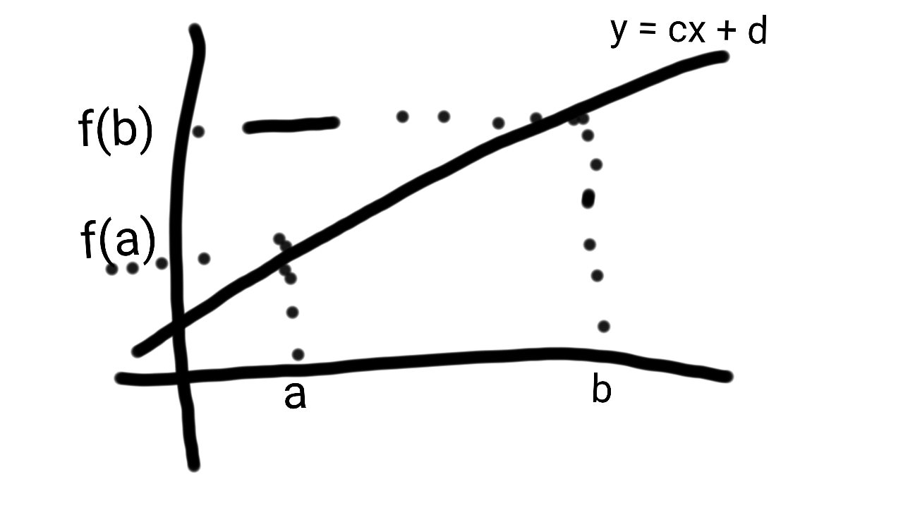
So with this, a function is a mapping from a set A to a set B, or in other words it is a subset of all combinations of ordered pairs whose first element is an element of A and second element is an element of B.

For example, if $A = \{ a, b \} \land B = \{ 1, 2, 3 \}$ then the combinations are: $F = \{ (a, 1), (a, 2), (a, 3), (b, 1), (b, 2), (b, 3) \}$ . A function f from A to B is denoted $f : A \rightarrow B$ and is a subset of F: $f \subseteq F$ .

This combination of pairs is called a Cartessian product, and is defined as the set: $\{ (a, b) \mid a \in A \land b \in B \}$ .

We have one more constraint to add to a function, namely that it cannot produce 2 or more different values for a single input. So using either of f(a) = 1 or f(a) = 2 or f(a) = 3 is okay, but not all three of them. That means that we only have to use one of $\{ (a, 1), (a, 2), (a, 3) \}$ from our example set above. The same reasoning goes for b. So $f = \{ (a, 1), (b, 2) \}$ with $f(a) = 1 \land f(b) = 2$ is one valid example.

We can also express recurrent relations like $f(x) = x \cdot f(x-1)$ for $f(0) = 0$ .

Conclusion

Matrices (tuples of tuples), lists (sets or tuples), graphs* (set of sets), digraphs (set of tuples), trees (graphs) can also be derived similarly.

This is what makes the set a powerful and interesting idea.

*: $G=(V,E)$ with vertices $V$ and edges $E$ . E.g.: $G = (\{a, b\}, \{(a, b), (b, b)\})$