To reach to here, we first had to work out the point slope formula and then figure out limits. Derivatives are very powerful. This post was inspired by doing gradient descent on artificial neural networks, but I won’t cover that here. Instead we will focus on the very own definition of a derivative.
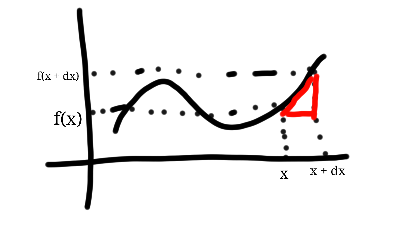
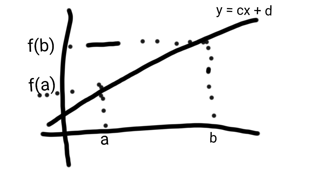
So let’s get started. A secant is a line that goes through 2 points. In the graph below, the points are and .
To derive a formula for this, we can use the point-slope form of a equation of a line: .
Plugging in the values, we get: .
What is interesting about this formula using the secant is that, as we will see, it provides us with a neat approximation at f(x). Let’s define . So now we have: .
The limit as dx approaches 0 for will give us the actual slope (according to the definition of an equation of a line) at x.
So, let’s define . This slope is actually our definition of a derivative. This definition lies at the heart of calculus.
The image below (taken from Wikipedia) demonstrates this for h = dx.
Back to the secant approximation, we now have: . This is an approximation rather than an equivalence because we already calculated the limit for one term but not the rest. As dx -> 0, the approximation -> equivalence.
For example, to calculate the square of 1.5, we let x = 1 and dx = 0.5. Additionally, if then . So . That’s an error of just 0.25 for dx = 0.5. Algebra shows for this particular case the error to be dx^2. For dx = 0.1, the error is just 0.01.
Pretty cool, right?
Here are some of the many applications to understand why derivatives are useful:
We can use the value of the slope to find min/max using gradient descent
We can determine the rate of change given the slope
We can find ranges of monotonicity
We can do neat approximations, as shown
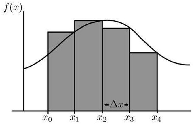
Integrals allow us to calculate the area under a function’s curve. As an example, we’ll calculate the area of the function in the interval . Recall that the area of a rectangle with size by is . Our approach will be to construct many smaller rectangles and sum their area.
We start with the case – two rectangles. We have the data points , which give us two rectangles with width and height and respectively – note the width is constant because the spaced interval is distributed evenly. To sum the area of this spaced interval, we just sum . But note that there’s an error, since the rectangles do not cover the whole area. The main idea is the more rectangles, the less the error and the closer we get to the actual value.
Proceed with case . We have the data points . Since we have four elements, in the range each element has width of . The result is .
Having looked at these cases gives an idea to generalize. First, note the differences of the points in – when , the difference between any consecutive points in is 1, and when , the difference is . Generalizing for , the difference between and will be . Also, generalizing the summation gives , and since we only consider evenly spaced intervals we have , for all . This is called a Riemann sum and defines the integral , where . Also, since is the starting point, that gives .
Going back to the example, to find the interval for , we need to calculate . From here, we evaluate the inner sum . Plugging back in gives .
Now we can take the limit of this as . Note that so we have , which finally gives . This represents the sum of the area under the curve of the function .
This post assumes knowledge in mathematical logic and algebra.
We will stick to sequences for simplicity, but the same reasoning can be extended to functions. For sequences we have one direction: infinity.
Informally, to take the limit of something as it approaches infinity is to determine its eventual value at infinity (even though it may not ever reach it).
As an example, consider the sequence . The first few elements are: 1, 0.5, 0.(3), 0.25, and so on.
Note that is undefined as infinity is not a real number. So here come limits to the rescue.
If we look at its graph, it might look something like this:
We can clearly see a trend that as x -> infinity, 1/x tries to “touch” the horizontal axis, i.e. is equal to 0. We write this as such: .
Formally, to say that , we denote: . Woot.
It looks scary but it’s actually quite simple. Epsilon is a range, N is usually a member that starts to belong in that range, and the absolute value part says that all values after that N belong in this range.
So for all ranges we can find a number such that all elements after that number belong in this range.
Why does this definition work? It’s because when the range is too small, all elements after N belong in it, i.e. the values of the sequence converge to it endlessly.
As an example, let’s prove that . All we need to do is find a way to determine N w.r.t. Epsilon and we are done.
Suppose Epsilon is arbitrary. Let’s try to pick N s.t. .
Let’s see how it looks for : for , we have: . This is obviously true since . So there’s our proof.
This bit combined with the slope point formula form the derivative of a function, which will be covered in the next post.
Lately I’ve been messing around with automated theorem provers. Specifically Prover9.
The moment you open it, if you use the GUI mode, you will see 2 big text boxes – assumptions and goals. Naturally, when playing one starts with simple stuff.
We leave the assumptions blank and set as our goal. If we click Start, we see that it proves it immediately.
% -------- Comments from original proof --------
% Proof 1 at 0.00 (+ 0.00) seconds.
% Length of proof is 2.
% Level of proof is 1.
% Maximum clause weight is 0.
% Given clauses 0.

1 P -> (Q -> P) # label(non_clause) # label(goal). [goal].
2 $F. [deny(1)].

============================== end of proof ==========================
That was fun, but what stood out for me is that in mathematics we often take axioms for “granted”, i.e. it’s rarely that we ever think about the logic behind it. But with Prover9, we need to express all of it using logic.
For Prover9 there is a general rule, that variables start with u through z lowercase. Everything else is a term (atom).
For start, let’s define set membership. We say denotes set membership, and that’s it. Because that’s all there’s to it, it’s like an atom. So let’s say that member(x, y) denotes that.
Now let’s define our sets A = {1}, B = {1, 2}, and C = {1}.
all x ((x = 1) <-> member(x, A)).
all x ((x = 1 | x = 2) <-> member(x, B)).
all x ((x = 1) <-> member(x, C)).
Now if we try to prove member(1, A), it will succeed. But it will not for member(2, A).
What do we know about the equivalence of 2 sets? They are equal if there doesn’t exist an element that is in the first and not in the second, or that is in the second and not in the first.
== is value check. For a and b to have the same value, we will say V(a, b). Thus a == b <=> V(a, b).
=== is value+type check. For a and b to have the same type, we will say T(a, b). Thus a === b <=> V(a, b) and T(a, b).
Now, to prove a === b => a == b, suppose that a === b. By the definitions, we have as givens V(a, b) and T(a, b). So we can conclude that V(a, b), i.e. a == b.
The contrapositive form is a != b => a !== b, which also holds.
However, note that the converse form a == b => a === b doesn’t necessarily hold. To see why, suppose a == b, that is V(a, b). Now we need to prove that V(a, b) and T(a, b). We have V(a, b) as a given, but that’s not the case for T(a, b), i.e. the types may not match.
So, whenever you see a === b you can safely assume that a == b is also true. The same holds for when you see a != b, you can safely assume that a !== b 🙂


![[0, 2]](https://s0.wp.com/latex.php?latex=%5B0%2C+2%5D&bg=ffffff&fg=000000&s=0&c=20201002)


![0.5 [ f(0.5) + f(1) + f(1.5) + f(2) ] = 2.5](https://s0.wp.com/latex.php?latex=0.5+%5B+f%280.5%29+%2B+f%281%29+%2B+f%281.5%29+%2B+f%282%29+%5D+%3D+2.5&bg=ffffff&fg=000000&s=0&c=20201002)


![[a, b]](https://s0.wp.com/latex.php?latex=%5Ba%2C+b%5D&bg=ffffff&fg=000000&s=0&c=20201002)
 . The first few elements are: 1, 0.5, 0.(3), 0.25, and so on.
 is undefined as infinity is not a real number. So here come limits to the rescue.
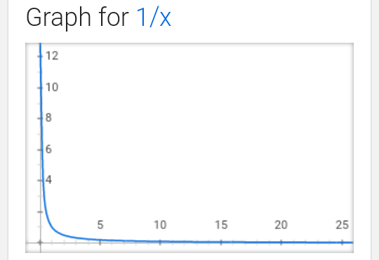
 .
. , we denote:
  . Woot.
 .
. : for
: for  , we have:
  . This is obviously true since
  . So there’s our proof.
 , this line passes through the point
  .
. .
.


 .
. as our goal. If we click Start, we see that it proves it immediately.
 denotes set membership, and that’s it. Because that’s all there’s to it, it’s like an atom. So let’s say that member(x, y) denotes that.