In Mathematics, there are many curves. From a constant curve 


Now, imagine that there is a huge data set with some points (think ordered pairs for simplicity), but not all points are defined. Essentially, machine learning is all about coming up with a curve (based on a chosen model) by filling gaps.
Once we agree on the model we want to use (curve we want to represent), we start with some basic equation and then tweak its parameters until it perfectly matches the data set points. This process of tweaking (optimization) is called “learning”. To optimize, we associate a cost function (the error or delta between the values produced by the equation and the data set) and we need to find for which parameters this cost is minimal.
Gradient descent is one algorithm for finding the minimum of a function, and as such it represents the “learning” part in machine learning. I found this video by StatQuest, along with this video by 3Blue1Brown to be super simple explaining these concepts, and naturally, this article will be mostly based on them.
In this article I will assume some basic set theory, and also derivatives. Further, through example, we will:
- Define what the curve (model) should be
- Come up with a data set
- Do the “learning” using gradient descent
The most scholar example to start with is the Body Mass Index. We will assume that it follows a linear curve, of the form 
The question now is, which linear function (of the form 


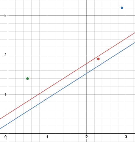
 (red),
  (blue), and the data points
In order to answer that question, we must first define what “best” means. We need to find a way to measure it. We state that every curve will have a “cost” with respect to the data set. Cost is defined as how well the curve fits the data set.
Residual sum of squares is one type of a cost function. It is defined as 
Let’s try it for 
So we want to somehow optimize the cost function 


Remember from high school that with derivatives we can find the critical point of a function, and in turn, determine the minimum/maximum points. To make our problem a little simpler we will assume 


The way the algorithm works is you start with a random point (value) for 

In other words, the algorithm is described by the formula 


To see the algorithm in action, here’s an implementation in Python based on Wikipedia’s example:
next_x = 6          # We start the search at x=6
rate = 0.01         # Step size multiplier
precision = 0.00001 # Desired precision of result
max_iters = 10000   # Maximum number of iterations
iteration = 0       # Initial
dg = lambda a: (279*a - 287)/10 # Derivative function

assert(iteration < max_iters) # Precondition
while iteration < max_iters:
    assert(callable(dg)) # Loop invariant I (before)
    current_x = next_x
    next_x = current_x - rate * dg(current_x)
    if abs(next_x - current_x) <= precision: break
    iteration += 1
    assert(callable(dg)) # Loop invariant I' (after), I=I'
assert(iteration == max_iters # Postcondition
  or abs(next_x - current_x) <= precision)

print("Minimum at %0.3f" % next_x) # 1.029
Now that we found out that 


ML is all about gathering data, running simulations, and making the best decision with the information available.
Pretty cool, right? 🙂

Thanks for sharing such valuable content here. This is the information which I was searching for. Machine Learning is the learning of computer’s language which is very trending nowadays. To enhance skills in Machine Learning visit Universal Informatics to have best Machine Learning Training In Indore.
LikeLike